Microsoft Excel 2013 comes with PowerPivot built in. To access PowerPivot tools, open Excel 2013 then open the ‘FILE’ tab, select ‘Options’ then ‘Add-Ins’. Look to the bottom of the ‘Add-Ins’ dialog and locate the ‘Manage’ drop down menu. Select ‘COM Add-ins’ and then click ‘Go’. Place a check mark next to ‘Microsoft Office PowerPivot for Excel 2013’, and while your there you might as well place a check mark next to the ‘Power View’ option.
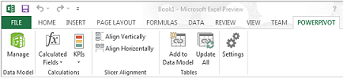
Now that you have turned on the PowerPivot Add-In, you will see the ‘POWERPIVOT’ tab on the Ribbon.
So, what can you do with PowerPivot that you can’t do with standard Pivot Tables? For starters, you’re not limited to the 1,048,576 rows of Excel. In fact your limit of rows is, well, way more. Second, you have the option to create data set links, allowing for one-to-many relationships across data sets. Third, you can now take advantage of the robust power of DAX functions. These functions are designed for speed, crunching through huge data sets in no time at all.
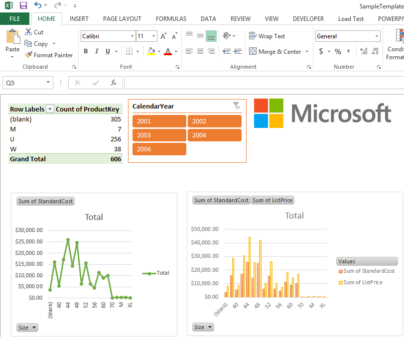
After you set up all your formulas, DAX functions and measures, you can now build KPIs, Pivot Tables, charts, Slicers and Timelines that make awesome, interactive data analysis dashboards. Your numbers will never look the same!