
VLookup. V stands for ‘Victory’. Well, not this time. It actually stands for ‘Vertical’. But, once you learn to use this popular function of Microsoft Excel, you WILL feel victorious.
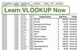
Use VLookup when you have two sets of data that you would like to turn into one. For instance: You may have a list of invoices of products purchased. You may also have a separate list of products on another Excel sheet. The challenge is to ‘marry’ these two lists, bringing the needed information from both lists into a single, complete list.
I have included a link to a file you can download so you can follow along as you read through this blog lesson. For your reference, the completed file is available for download as well.
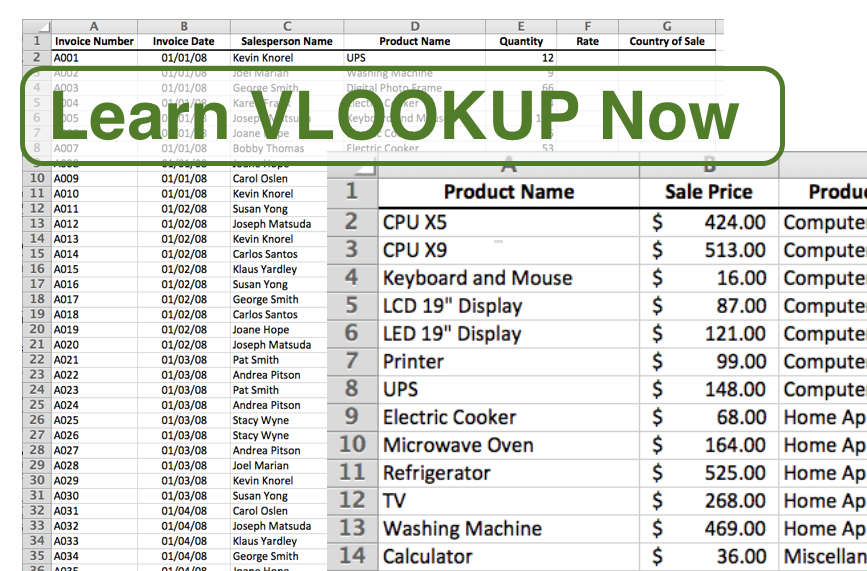
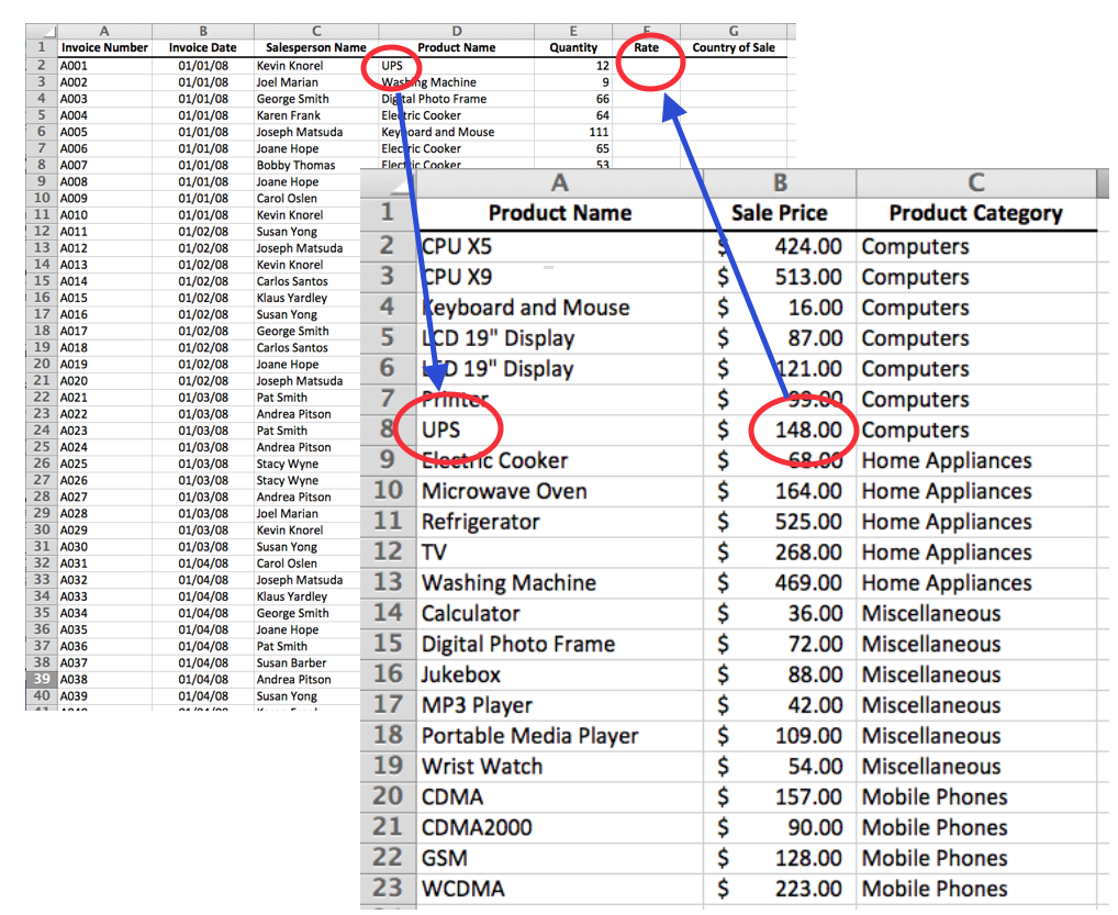
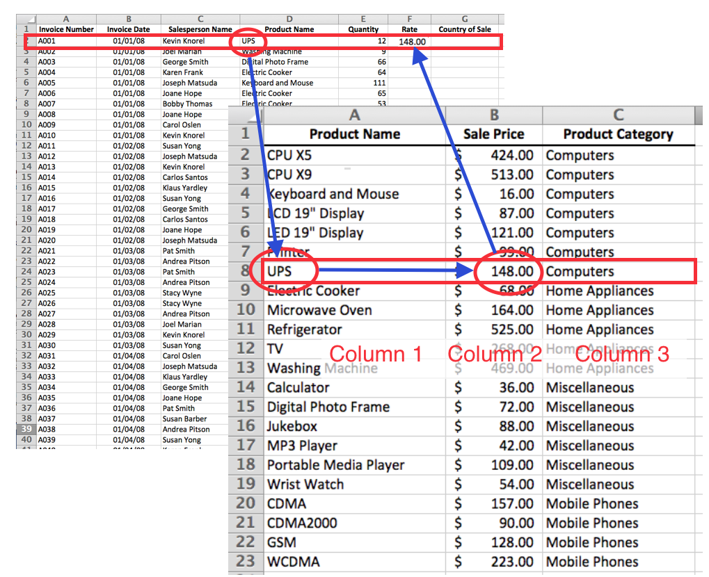
In this example we will use VLookup to bring the Sales Price from the Products list over to the Invoices list Rate column. We will use the Product Name in the Invoices list to ‘look up’ the same Product Name in the Products list.
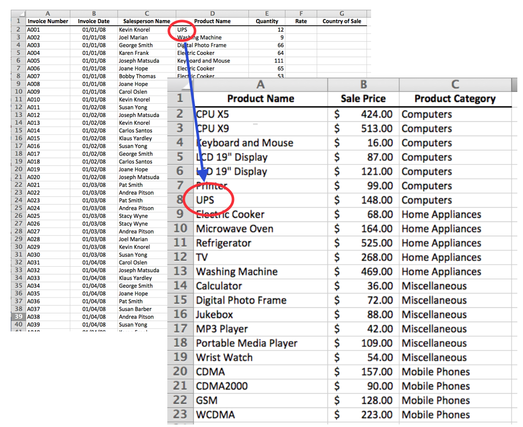
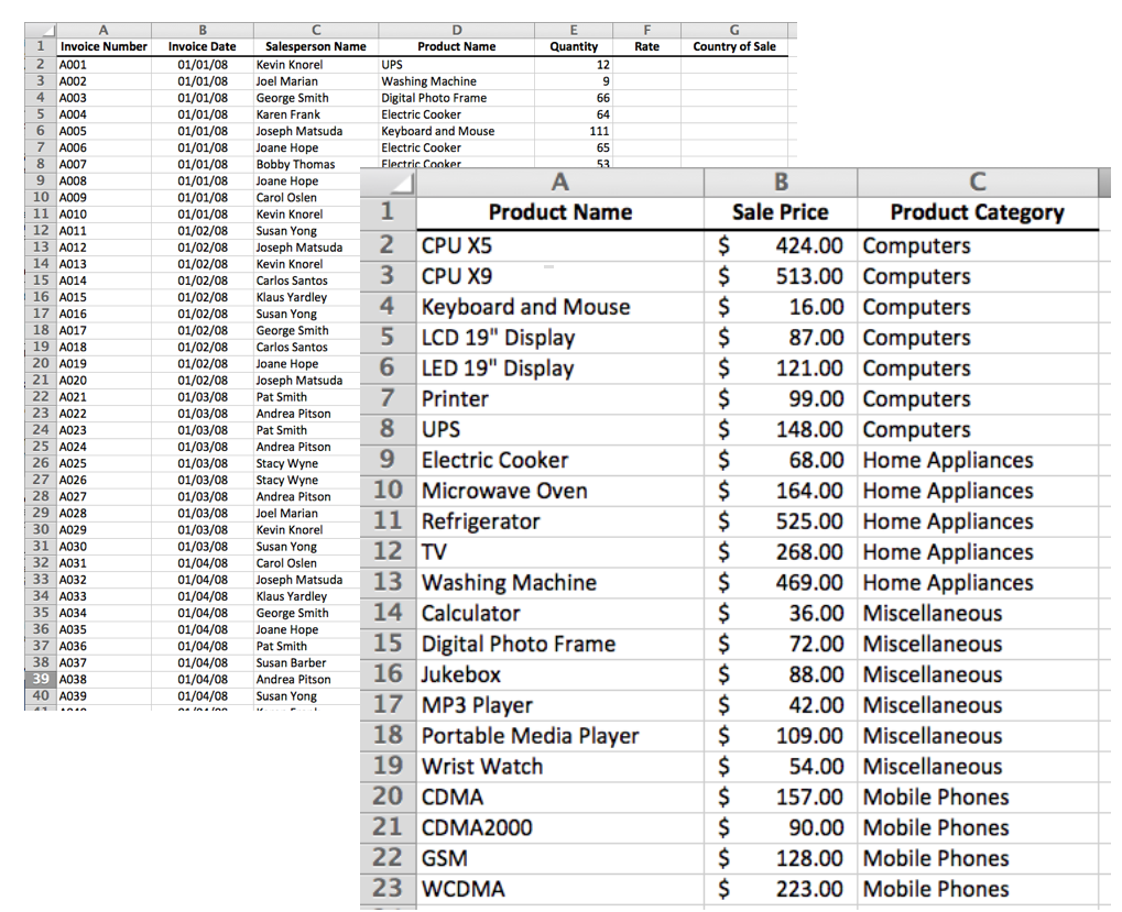
Once we find the correct product name, we can ‘index’ over to the Sale Price column and send it back to the Invoices list Rate column. In this case invoice ‘A001’ shows a ‘UPS’ unit was purchased. Take a look at the Products list and notice ‘UPS”, glance over to column 2 and see the price for a UPS is $148. Now we will put the $148 into invoice line A001 under the Rate column.
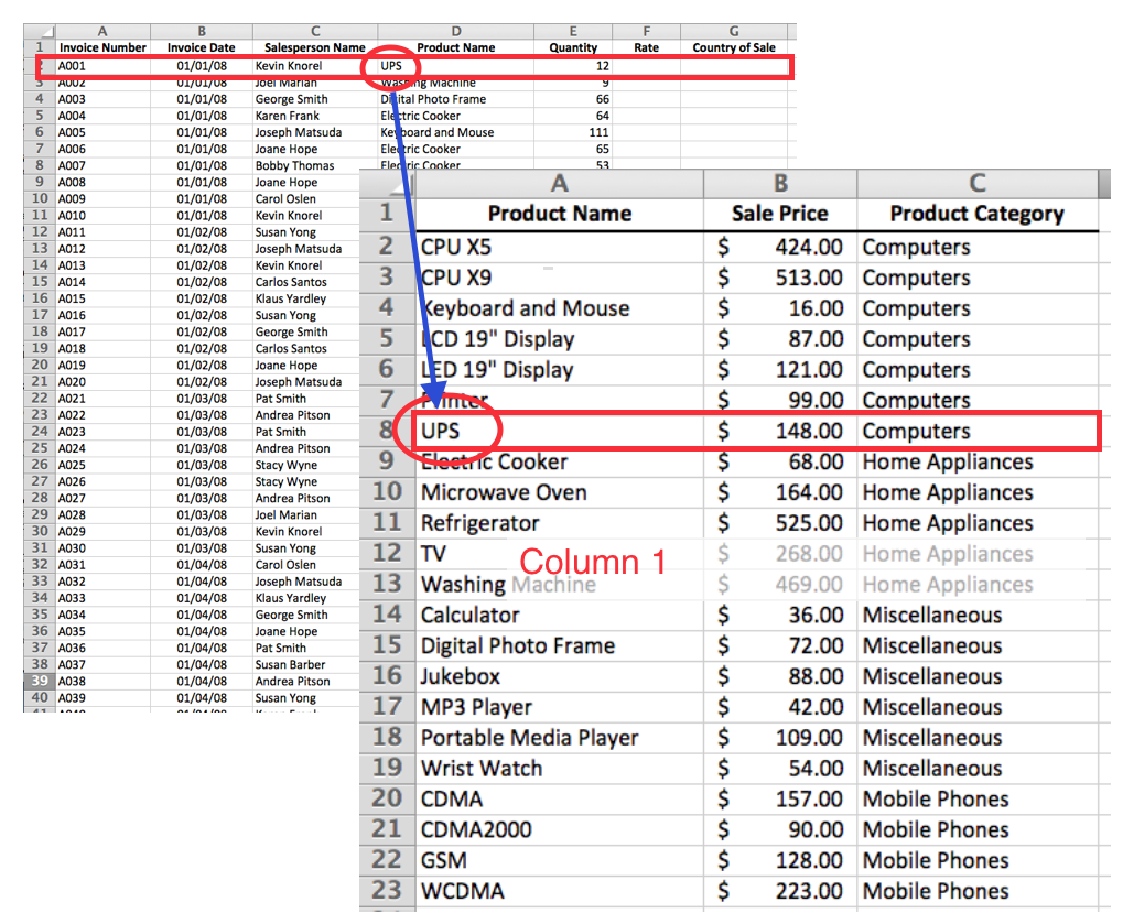
To start a VLookup formula, we must first reference the cell we want to “look up”. In this case we will look up cell D2 in the Invoice list and compare it to the first column (column 1) in the Products list. The ‘vertical’ aspect of VLookup refers to the fact that VLookup will start looking from the top of column 1 in the Products list and continue looking down (vertically) until it finds a match.
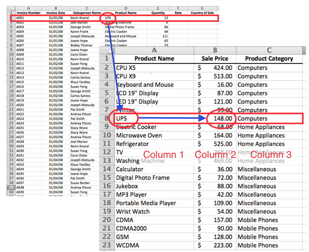
When a match is found, we then instruct VLookup to ‘index’ over to the column we would like to return to the Invoice list. Since we are looking to find the Sale Price/Rate of the Product, we specify column 2. (If we wanted to return the corresponding Product Category we would specify column 3)
There is one more part of the VLookup we must consider. VLookup has two modes of operation: True and False. Think of this as a question: “Is this a RANGE lookup?” In other words are we looking for a product name that is similar to “UPS”, or are we looking for “UPS” exactly? We are looking for an EXACT match, not a ‘close enough’ match. So in this example, the answer would be FALSE to the question: “Is this a range lookup?”
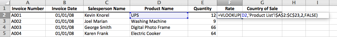
Carolyn, here is the VLookup formula entered into cell F2 of the Invoices list:
=VLOOKUP(D2,‘Products List’!$A$2:$C$23,2,FALSE)
D2 is the relative cell reference we want to look up
‘Products List’!$A$2:$C$23 is the absolute range where VLookup will find the information on the Products sheet in cells A2:C23
2 refers to the 2nd column in the lookup table. This is the column we want to send back to Invoices when a product match is found
FALSE instructs VLookup to find an exact match, not simply a ‘close’ match
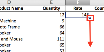
 Now that you have the formula entered into cell F2, use the Autofill Handle on the lower right corner of F2 (the active cell) and double click (or drag) to copy the formula to the bottom of the list.
If you downloaded the exercise file for this lesson, you will notice that I have included a ‘Salesperson List’ sheet for you to practice VLookup. Using what you have learned, try to build a VLookup formula to look up the Country of Sales and bring it to the Invoice sheet.
Here is the formula if you want to check your work:
=VLOOKUP(C2,’Salesperson List’!$A$2:$D$17,3,FALSE)
I have included a link to a file you can download, so you can follow along as you read through this blog lesson. For your reference, the completed file is available for download as well.
Enjoy the sweet taste of Victory.